
What’s my house worth? - Building a full stack Flask app
This blog post documents my first foray into developing a full stack analytical pipeline to administer a machine learning solution including using AWS tools such as EC2, S3 and RDS for backend infrastructure and Flask for front end UI. Furthermore, through this project, I got exposure to several good software engineering practices like testing, modularility, reproducibility, logging, managing dependencies, versioning and agile software development paradigm.

PROJECT CHARTER
VISION
Real estate agencies require accurate estimation of the price of a property to decide whether it is undervalued or not before making an investment decision. Individual home buyers also need an objective estimate of a home before buying. House pricing decisions are often subjective and can lead to bad investment decisions. The vision is to develop a platform which would help estimate the price of a property based on certain property characteristics to help drive investment decisions, increase profits and reduce costs.
MISSION
The mission of this project is to build an app which would help accurately predict the price of a property based on certain characteristics like property type, no. of floors, age etc. which can be deployed as a website as well as an Android/iOS app.
SUCCESS CRITERION
Modeling ACCURACY: The model is successful if the modeling accuracy (R-square evaluation metric) exceeds 60%
BUSINESS OUTCOME: A Key Performance Indicator of the success of the app would be continual increase in it’s adoption to drive business decisions by the various Real Estate agencies and individual customers. This would be a good indicator of the model’s accuracy performance as well. The intention is to deploy the app at a particular location, and based on the performance expand to other areas.
PROJECT PLAN
Since we had to simulate working in a agile software development paradigm, the following project plan was constructed and the work was divided across two sprints of two weeks each.
THEME: Develop and deploy a platform that helps estimate the valuation of a property based on certain characteristics
- EPIC 1: Model Building and Optimization
- Story 1 : Data Visualization
- Story 2 : Data Cleaning and missing value imputation
- Story 3 : Feature Generation
- Story 4 : Testing different model architectures and parameter tuning
- Story 5 : Model performance tests to check the model run times
- EPIC 2: Model Deployment Pipeline Development
- Story 1 : Environment Setup : requirement.txt files
- Story 2 : Set up S3 instance
- Story 3 : Initialize RDS database
- Story 4 : Deploy model using Flask
- Story 5 : Development of unit tests and integrated tests
- Story 6 : Setup usage logs
- Story 7 : Solution reproducibility tests
- EPIC 3: User Interface Development
- Story 1 : Develop a basic form to input data and output results
- Story 2 : Add styling/colors to make the interface more visually appealing
Sprint Sizing Legend:
- 0 points - quick chore
- 1 point ~ 1 hour (small)
- 2 points ~ 1/2 day (medium)
- 4 points ~ 1 day (large)
- 8 points - big and needs to be broken down more when it comes to execution (okay as placeholder for future work though)
Sprint Plan:
Sprint 1:
- EPIC 2 : Story 2 : Set up a S3 instance (1)
- EPIC 2 : Story 3 : Initialize RDS database(1)
- EPIC 1 : Story 1 : Exploratory Data Analysis (2)
- EPIC 1 : Story 2 : Data Cleaning and missing value imputation (2)
- EPIC 2 : Story 1 : Environment Setup : requirement.txt files (1)
Sprint 2:
- EPIC 1 : Story 3 : Feature Generation (2)
- EPIC 1 : Story 4 : Testing different model architectures and parameter tuning (8)
- EPIC 1 : Story 5 : Model performance tests (2)
- EPIC 2 : Story 4 : Deploy model using Flask (2)
- EPIC 2 : Story 5 : Development of unit tests and integrated tests (4)
- EPIC 3 : Story 1 : Develop a basic form to input data and output results (2)
- EPIC 2 : Story 6 : Setup usage logs (2)
- EPIC 2 : Story 7 : Solution reproducibility tests (4)
IceBox:
- EPIC 3 : Story 2 : Add styling/colors to make the interface more visually appealing
REPO STRUCTURE
The Cookiecutter project structure template was considered for the repo structure. The reason why this was used is that it provided a logical, reasonably standardized and flexible project structure to work with. The repo structure is illustrated below:
├── README.md                         <- You are here
│
├── app
│   ├── static/                       <- CSS, JS files that remain static
│   ├── templates/                    <- HTML (or other code) that is templated and changes based on a set of inputs
│   ├── app.py                        <- Contains all the functionality of the flask app
│
├── config                            <- Directory for yaml configuration files for model training, scoring, etc
│   ├── logging_local.conf            <- Configuration files for python loggers
│   ├── config.py                     <- Contains all configurations required for processing and set up
│   ├── flask_config.py               <- Contains all config required for the flask app
│
├── data                              <- Folder that contains data used or generated. Not tracked by git
│   ├── raw/                          <- Place to put raw data used for training the model
│   ├── clean/                        <- Contains the cleaned dataset after the raw data has been cleaned
│   ├── features/                     <- Contains the data with the features
│
├── database                          <- Folder that contains the local SQLite database
│
├── deliverables                      <- Contains all deliverables for the project
│
├── logs                              <- Contains execution logs
│
├── models                            <- Trained model objects (TMOs), model predictions, and/or model summaries
│
├── notebooks
│   ├── develop                       <- Current notebooks being used in development
│   ├── deliver                       <- Notebooks shared with others
│   ├── archive                       <- Developed notebooks no longer being used
│
├── src                               <- Contains all the scripts for the project
│   ├── archive/                      <- No longer current scripts.
│   ├── helpers/                      <- Helper scripts used in main src files
│   ├── load_data.py                  <- Script for downloading data from the input source
│   ├── clean_data.py                 <- Script for cleaning the raw data
│   ├── features.py                   <- Script containing features that are required to be generated for modelling
│   ├── generate_features.py          <- Script that uses the features script to generate features
│   ├── log_usage_data.py             <- Script for building the usage log database and injesting data in it
│   ├── train_model.py                <- Script that trains the model using the final training data
│
├── tests                             <- Contains files for unit testing
│
├── run.py                            <- Simplifies the execution of one or more of the src scripts
│
├── requirements.txt                  <- Python package dependencies
│
├── Makefile                          <- Makefile to execute the make commands
DATA DETAILS AND EXPLORATORY DATA ANALYSIS
DATA DETAILS
The popular Ames housing dataset was used for this analysis (source: Kaggle). The dataset contains details of 1,460 properties from Ames, IA region and their sale prices. House attributes included 79 variables including zoning characteristics, neighbourhood details, quality scores, utilities, build year, whether remodeled etc. Looking at data completeness, I observed that there were a few variables that have a very high percentage of missing values. A quick look at the data dictionary revealed that this data was structurally missing, and hence was imputed appropriately. Eg. 93.7% of the records had missing values for the field Alley. This implied that 93.7% of all the houses did not have alley access. Similarly, 5.54% of houses in our dataset did not have a garage. All these values were imputed by either 0 or None wherever appropriate.
EXPORATORY DATA ANALYSIS
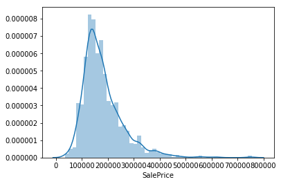
The house prices in the dataset ranged from $35,000 to $750,000. A quick look at the target distribution (Figure 1) reveals that majority of houses had prices between $80,000 and $400,000. The target distribution was fairly normally distributed with a slight right skew.
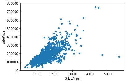
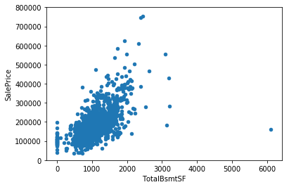
Next I looked at scatterplots to understand the relationships between the target and a few numerical variables present in the dataset. Figure 2 shows the scatterplots of the target with GrLivArea (Total above ground square footage) and TotalBsmtSF (Total Basement square footage). Both the plots show that the target is positively related to both the variables.
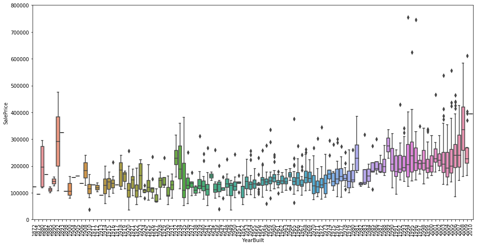
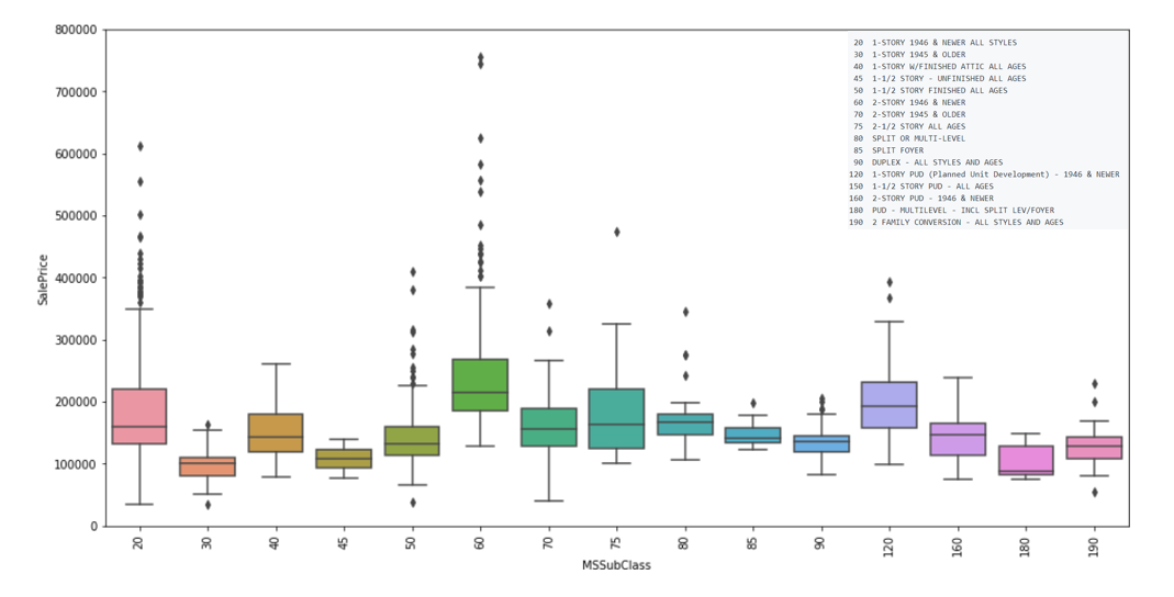
Further, I was interested in understanding whether the time of build of a house impated its sale price. The below boxplots illustrate the relationships between the variables YearBuilt and MSSubClass. Looking at the plots, we can see that the year of build did not necessarily have any impact on the price of the house. Hwowever, the variable MSSubClass revealed a different story. It can be seen that houses built after 1946 had on average higher prices that older built houses.
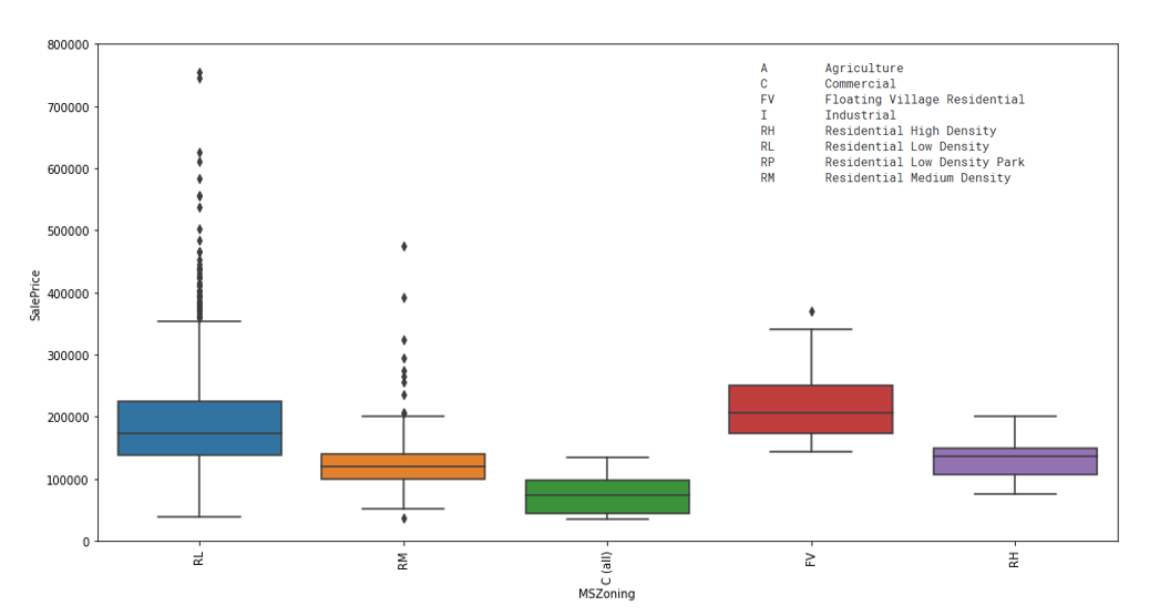
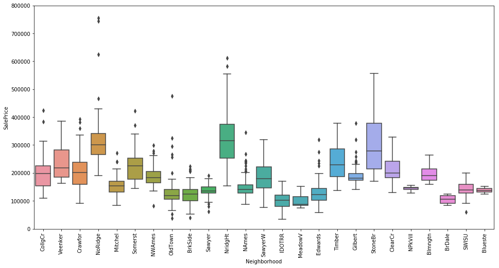
Another hypothesis was that the neighbourhood characterstics could potentially impact the sale price. The below boxplots illustrate the relationships between the variables MSZoning and Neigbourhood. From both the plots, we can clearly see that certain neighbourhoods or type of neighbourhood have higher sale prices as compared to others.
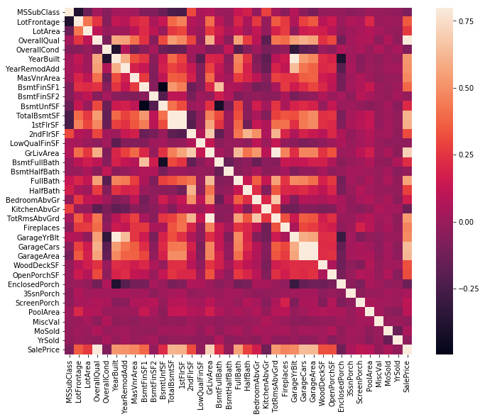
Looking at the correlations of our response variable SalePrice with all the variables (Figure 5), we can see that the highest correlations are with OverallQual, GrLivArea (Above ground living area), TotalBsmtSF (Total Basement Area), 1stFlrSF (First floor area), FullBath (Full bathrooms above grade), GarageCars and GarageArea. Furthermore, the following set of response variables have high correlations between them:
- TotalBSMTSF and 1stFlrSR
- GarageCars and GarageArea
- GarageYrBuilt and YearBuilt
- TotRmsAbvGrd and GrLivArea
Most of the above combinations make sense. E.g. GarageCars and GarageArea are highly correlated. This is intuitive as the number of cars that a garage can accomodate will be a function of the total area available. Including both variables amongst the above sets in our model may lead to multi-dimensionality problems while modeling; however since we use a tree based model for modeling, we do not run into this problem.
MODELING
DATA CLEANING & FEATURE GENERATION
The target was to predict the SalePrice using the other variables. The following variables were dropped from the training data: YearRemodAdd, MiscVal, MoSold, YrSold, SaleType and SaleCondition. The categorical variables were converted to one-hot encoded dummy variables. A new binary variable called RemodelledFlag was constructed depending on whether the house had undergone remodeling or not.
MODEL BUILDING
For modeling, the sklearn implementation of the Random Forest Regressor was used. For the first iteration, all the variables were considered for modeling. Grid search hyperparameter optimization was used to identify the best combination of hyperparameters (max_depth and max_features) optimizing for the OOB (out-of-bag) R-square score. The number of trees were fixed at 1000. The best performing model had max_depth as 22 and max_features as 210 and an OOB R-square of 85.95%. The feature importance plot was evaluated to identify the most impactful variables. It was observed that except a few, most of the variables had very low to no contribution to the model. The model was refit using only the features having feature importances > 0.005. The feature OverallQual although being the most impactful was dropped from the model as quality scores were subjective and not an intrinsic characteristic of a house.
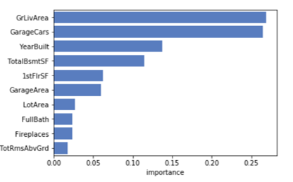
The model was retrained using the reduced list of features. The final model contained the following 10 variables:
- GrLivArea
- GarageCars
- TotalBsmtSF
- YearBuilt
- 1stFlrSF
- GarageArea
- FullBath
- LotArea
- TotRmsAbvGrd
- Fireplaces
Since the number of variables were reduced, hyperparameter optimization was again performed to derive the best performing hyperparameters. The best performing model had max_depth = 16 and max_features = 6 with n_estimators fixed at 1000. It had a OOB R-square score of 82%. Since this satisfied our modeling success criteron, this was finalized as the final model object. The model object was saved as a pickle file to be integrated into the full pipeline. Figure 6 highlights the feature importances for the final model.
MODELING PIPELINE
The app has been configured to run in two different modes: Local and AWS depending on the infrastructure requirements. Please refer to the project README for full set of instructions of how to setup the app.
The following figure depicts the full modeling pipeline:
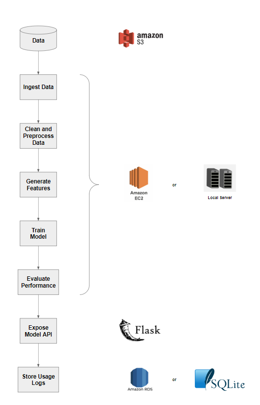
The raw data for this project has been downloaded and uploaded to an open S3 bucket. Depending on the mode, the compute engine can be a local server for mode = ‘Local’ or an EC2 instance for mode = ‘AWS’. The compute engine will fetch the data from the S3 bucket, clean the data, generate features, train and evaluate model and launch the flask app. The model parameters are defined in config/config.yml. The app usage information will be logged in a sqlite database (mode = ‘Local’) or a RDS database (mode = ‘AWS’). The usage information can be analyzed for tracking and analyzing app adoption.
An user interface was developed using HTML and CSS to provide a user friendly interface to interact with the model API. The following figure depicts the UI:


APP DEVELOPMENT ASPECTS AND LEARNINGS
MODULARITY
Modularity refers to the extent to which a software/Web application may be divided into smaller modules. Every element of the modeling pipeline was controlled by its own submodules within the app. This allowed me to develop and test individual components independently which made debugging and scope of further development easier.
TESTING
Unit Tests were built in to test individual functions. All tests reside in the tests/ folder. Unit tests help us understand whether the functions are behaving as desired and help prevent untowardly bugs. It is important to have testing built in specifically in production systems to ensure that the system is behaving as desired.
LOGGING
The default python logging package was used for logging purposes. All logging configurations are controlled via theconfig/logging_local.conf file. The different logging modes (info, debug, error) have been extensively used during development and deployment to debug and keep track of progress. Having descriptive logging messages throughout the code helped me understand what my code was doing and identify bugs, changes in functionality, input data quality, and more.
REPRODUCEABILITY
Machine Learning solutions need to be reproduceable. This means that anyone having access to the code should be able to replicate the model performance metrics that have been reported for the model. This is important to validate the performance and gain trust and buy-in from the model consumers. In order to ensure that anyone can replicate the modeling pipeline, a Makefile was built to execute the entire pipeline. A Makefile is a file containing a set of directives used by a make build automation tool to generate a target/goal.
ACKNOWLEDGEMENTS
Sincerest thanks to the following for helping me throughout the project:
- Tanya Tandon (QA)
- Chloe Mawer (Course Instructor)
- Fausto Inestroza (Course Instructor)
- Xiaofeng Zhu (Course TA)


Leave a comment