
Helping an Online bookstore quantify the impact of their promotion strategy
The goal of this project was to predict whether a given customer will respond to a promotional email sent out by an online bookstore, and how much they will spend on buying books if they do respond.

We were given a scenario where an online bookstore decided to reach out to customers via email as a promotional activity to increase sales. For our analysis, we were provided past history of all the bookstore’s customers and their response to an earlier conducted promotional activity. Our assumption was that the past buying history of a customer was indicative of whether he/she will respond to this promotional activity or not. Several feature indicating buying patterns were constructed and evaluated to understand the customer behaviour. We focused on the importance of the “time factor” in numerous ways in our analysis, hypothesizing that partitioning data based on date ordered would prove extremely beneficial. Our section on data cleaning and exploratory data analysis details our methods for creating these time-sensitive variables, along with their interactions, in the hopes of creating a successful predictive model.
Another goal of ours involved exhaustively searching the large feature space for any indicative features, knowing that we could rely on stepwise selection to reduce the number of predictors to the most significant subset. We had information on the category of books (Art, music, fiction etc.) ordered by the customers. Constructing features centered around each of these categories led us to have > 60 features in our initial model. In order to separate the grain from chaff, we utilized the random forest algorithm for selecting the most impactful variables. This analysis is detailed at the beginning of our model fitting section. After narrowing down which category variables are the most significant, we moved on to building the core of our analysis: our predictive models. Our model fitting section discusses our methods to create optimized logistic regression and multiple linear regression models, including outlier removal, model diagnostics such as Cook’s distance and VIF calculation, and stepwise selection. Finally, we discuss the accuracy of our models, both statistically and financially.
DATA CLEANING AND EXPLORATORY DATA ANALYSIS
The data provided consisted of two datasets. The first dataset contained information at a customer level which included recency of purchase, frequency of purchase, total time on file, and recency and frequency metrics for individual book categories (Fiction, Classic, Cartoons etc.). Inforation for 30 different category types was provided. The second dataset contained order level information wherein we had data on order date, caategory of boks ordered, quantity and amount. The target was provided as the log of total amount spent (logtargamt) by the customer as a response to the promotional activity.
Our goal regarding data cleaning and exploratory data analysis involved identifying, combining and partitioning variables that we hypothesize to be potentially significant predictors. We first endeavoured to pinpoint significant information, if any, contained in the category variables. These variables proved cumbersome due to their sheer number. Rather than abandoning these variables, we looked into ways to reduce their dimensions by examining the relationships between categories. To begin, we looked at the correlation matrix (Figure 1) between the category amount variables.
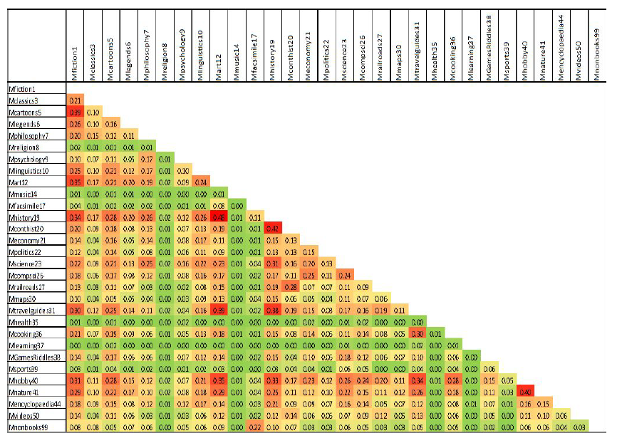
No correlations were very high, with the highest correlations between certain category variables being slightly less than 0.50, but in the amount correlation matrix, we were able to identify some categories which seemed to be related, with a correlation greater than 0.3 considered as significant. It was observed that the following categories were intercorrelated: Fiction, Cartoon, Art, History, Travel Guides, Hobby, Contemporary History, and Nature. In our feature engineering steps, we created a variable Mgroup, adding together the amount values for these categories, and the variable Fgroup, adding together the frequency values for these categories.
Observations regarding individual orders and order pricing, namely that sometimes a single book can cost upwards of $1000, caused us to question the significance of the “amount” variable representing the total amount spent by a single customer summed across all order data. Therefore, we created a separate variable, qty, representing the total number of books bought by a single customer summed across all order data. Dividing the qty variable by time on file yielded a useful interaction that we later included in both the logistic and linear regression models. Additionally, we created a variable called amount upon quantity that created another metric comparing dollar amount and quantity of books by dividing amount by qty. Other interaction variables created included: dividing amount by total number of orders , dividing qty by frequency, and dividing frequency by time on file.
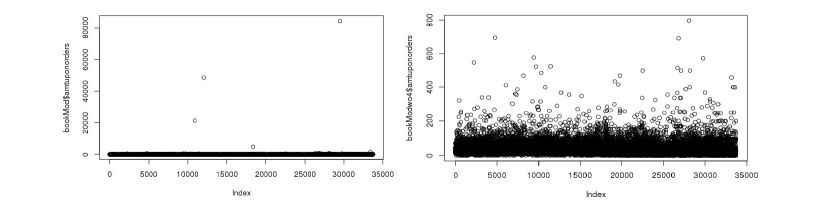
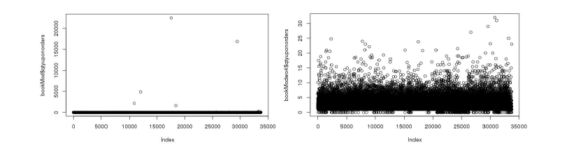
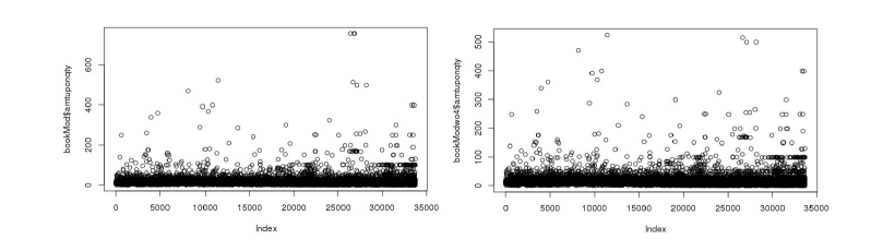
For dealing with outliers, we created three criteria based on some of the interaction variables mentioned above. We removed observations where:
- Amount divided by the total number of orders (amtuponorders) exceeded $1000
- The total number of books per total number of orders (qtyuponorders) exceeded 40
- Amount divided by total number of books ordered (amtuponqty) exceeded $600
Overall these three criteria only removed 0.0355% (12 observations) of the total data, while improving the fit of our two models on the training data. While we cannot be certain that these data are incorrect, our goal was to create the most accurate model while not mispredicting large values in the test data, and these criteria best struck that balance. The scatterplots for the variables both before and after outlier removal are illustrated in Figure 2. Later on, for our multiple linear regression model, we used Cook’s Distance to identify a few more outliers.
Much of the data relies on time to chart consumer behavior, and we intended to capture the effect of the time an order is placed on the response variable. While the recency variable charts the number of days since the most recent order a customer has placed, the order date variable records the date of all orders a customer has placed. We utilized information about both the most recent order and the total orders, per customer, to build a number of novel features in the hopes of illuminating relationships between time and targeted amount. We separated customers by timeframe of order, partitioning customers into groups based on who had ordered in the last 1, 3, 6, and 12 months. Summary statistics for each group, by customer, were calculated, namely quantity of books ordered in this time frame, designated qty, and total dollar amount, designated price. Thus, we were able to separate the two variables discussed in the previous paragraph, amount and qty, into a few time-frame partitions. When considering the total number of orders per customer, we were able to calculate the percentage of the total amount purchased, per customer, that occured in these time frames. Therefore, we were able to observe sale trends for each customer over the past year.
When organizing customers based on order date in this manner, we decided to order time on file in a similar way. Partitioning customers based on time on file in the last 1, 3, 6, and 12 months gave us a separation between newer and older customers. During this analysis of time on file, we discovered an interesting observation about a small subset of the customers. In the training set, 87 individuals have a time on file value of zero; similarly, 271 individuals in the test set have a time on file value of zero. These customers are brand new to the online store database; therefore, they have no previous order data and so would be nearly impossible to create accurate predictions for. We were unable to remove these observations due to 52.9% of the new customers in the training set being responders. Since the overall percentage of responders in the dataset is 3.93%, removing the new customers would remove a significant portion of the responders. We therefore decided to manually impute predicted values for these observations. The imputation process will be detailed in the next section, as it is different for the logistic and the linear regression models.
MODELING
RANDOM FOREST VARIABLE SELECTION ON BOOK CATEGORIES
We ran two random forest models in order to identify potentially important book category variables with respect to classifying responders and predicting log-target amount. The input variables include frequency as well as amount variables for each category (60 variables in total). The output variable is a binary flag capturing whether a customer bought a book (logtargamt equals 0 or not) for the classification model, and logtargamt (for the subset of data that only contains responders) for the regression model. Library caret was used to tune both the classification and the regression random forest models.
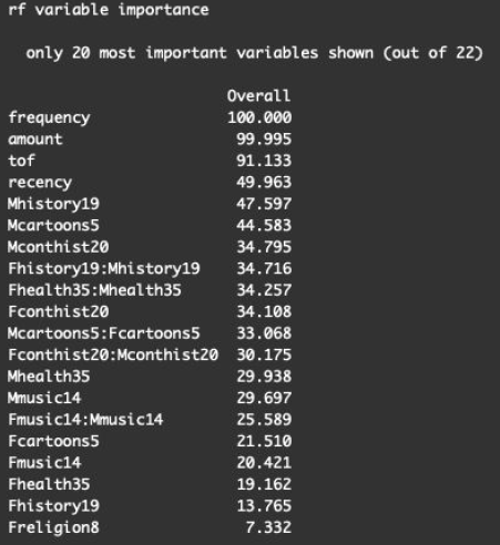
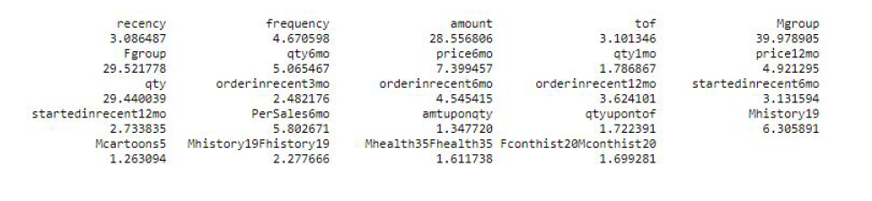
The random forest analysis provided us with a few important category variables that accurately classified and predicted the customers’ purchasing propensity. The CCR (Correct Classification Rate) for the category-only classification model is 0.9625, slightly better than the null model (classifying everything to the category of logtargamt = 0, with a CCR of 0.9606) indicating that adding some categories might provide valuable information to our logistic and linear regression models. To identify the important category variables, we ran the variable importance function within the caret package and selected the top 6 categories that were reported as highly important (with an importance score larger than 30) in both the classification and the regression model. We included these variables in our initial logistic and linear regression models.
We also created interaction terms between the frequency and amount for each aforementioned important category in order to capture any interaction effect. These interaction terms were added to the preliminary logistic and linear model fitting as well. A graph showing the final important categories selected by random forest is shown in Figure 3.
CLASSIFICATION MODEL: BINARY LOGISTIC REGRESSION
To create a logistic regression model, the response variable received the necessary transformation into a binary variable. This binary variable has a value of 1 if logtargamt > 0 and a value of 0 if logtargamt = 0. Our preliminary model included all the variables we created, in addition to the recency, frequency, amount, and time on file variables that were included in the original dataset. These included the time-related variables we had created - total quantity, dollar amount, binary flag if any orders have been placed in given time frame, and time on file in given time frame - for 1 month, 3 months, 6 months, and 12 months, in addition to our qty variable and the numerous interaction variables we created. We also included the Mgroup and Fgroup aggregated category variables along with the most significant category variables as found through our random forest model.
As stated in the previous section, the customers with a 0 value for time on file (i.e. brand new customers) did not have data related to previous orders, rendering it near impossible to predict their target amount. This necessitated a manual imputation method of predicted values. For this logistic regression, we decided that the response rate for the new customers in the training set (0.5287) adequately replaced the probability of logtargamt > 0 for these new customers. Since this manual imputation replaces the predictive model for new customers, we removed all new customers from both the training and the test set before performing the logistic regression. The new customers from the test dataset were placed back into the dataset later when validating our predictive model with the imputed value 0.5287 serving as the predicted probability.
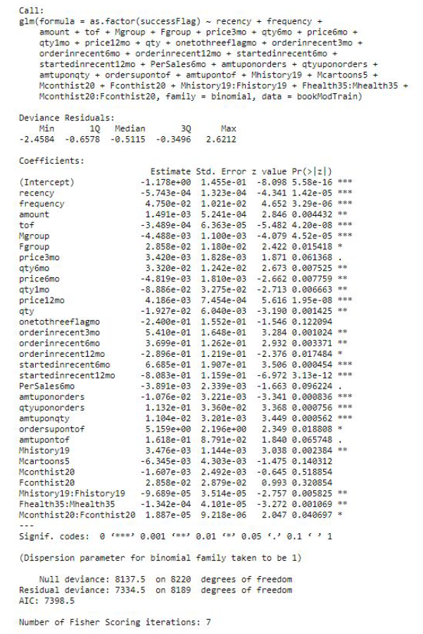
Since the response rate for the training data was very low (3.93%), we utilized bootstrapping to oversample the responders (customers with logtargamt > 0) to ensure the validity of our model in predicting customers as responders. We assigned weights for each responder and non-responder in the training data and sampled with replacement to get our final training set. The percentage of responders in the final dataset is 20% and non-responders is 80%. The dimensions (number of observations and variables) of the final training data is the same as the original training data. We ran backward stepwise regression with 42 variables minimizing AIC to arrive at an optimal model. The initial model summary has been presented in Figure 4.
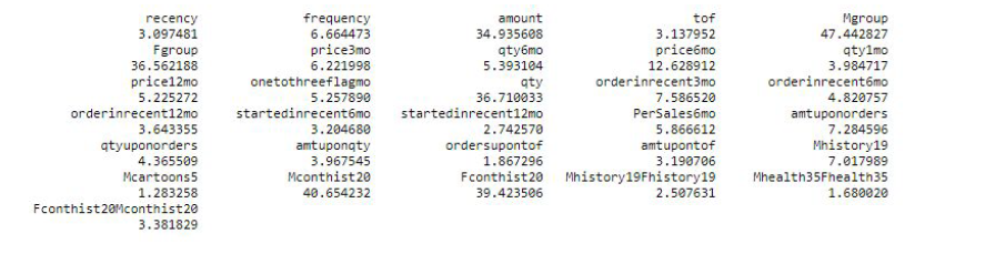
We checked the variance inflation factors for the final predictors and removed the variables that had VIF values significantly larger than 10 and low predicting power in the model. Note that we did not remove the variables Mgroup and Fgroup since they are highly significant at the 5% level in classifying responders, even though they had VIF values above 30. Please also note that we removed the variable amount even though it was significant in the original model. After removing variables with high inflation values, amount became non-significant at 5% level, suggesting multicollinearity with some of the removed variables, so we removed the amount variable as well. We refit the model with the remaining predictors after removing these variables and arrived at our final model. The final model is summarized in Figure 5.
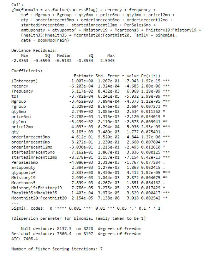
In our final logistic regression model, recency, frequency and tof are all highly significant (at 1% level) in classifying response. Variables capturing customer purchasing behavior, including whether a customer purchased in the recent 3, 6, 12 months, whether a customer just started in the recent 6, and 12 months are also all highly significant. Moreover, the interaction term between customers’ purchasing amount and quantity and the interaction between quantity and time of file are also very important in classifying response. In terms of book category variables we added to the model, Mgroup and Fgroup proved to be statistically significant at the 1% level, in addition to the amount variable for History and Cartoon, the interaction between the amount and frequency variables for History, the interaction between the amount and frequency variables for Contemporary History and the interaction between the amount and frequency variables for Health. The final number of variables in our logistic model is 23 out of the original 42. The residual deviance is 7360.4 on 8197 degrees of freedom and the final AIC is 7408.4. We also tried fitting the model without the bootstrap oversampling on responders, which generated a much lower AIC of around two thousand. However, since the model without bootstrap classified most customers into non-responders and has low predicting power on responders, we decided to use the model with bootstrap as our final model.
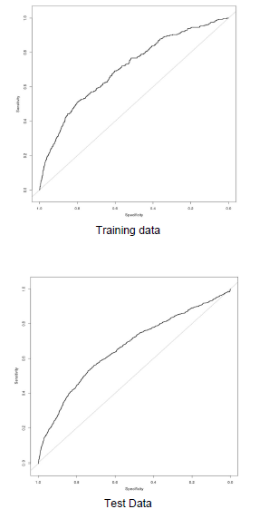
We graphed the Receiver Operating Characteristic curve for our final logistic model using the training as well as the test data, as is shown in Figure 6. The curve deviates from the 45 degree line by a significant amount, suggesting that our model has good predicting power. The area under the ROC curve is 0.70 for training data and 0.66 for the test set, which shows that our model is decently accurate in classifying responders and non-responders, but also did not blindly classify everyone as non-responders.
MULTIPLE LINEAR REGRESSION MODEL
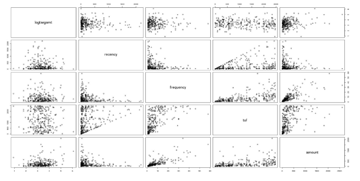
In the logistic regression model, we did not worry about the varying purchase amount; we merely wished to predict whether a customer would respond to the promotion and purchase anything at all. However, building the multiple linear regression model necessitated further exploration of the spread of the target amount variable. We first explored the subset of our training dataset where logtargamt was greater than zero and time on file is greater than zero (customers who responded to the survey and also have previous order data). This left us with 280 observations. We began with a number of scatterplot matrices which plotted the relationship between logtargamt and the variables provided in the training dataset (Figure 7). This gave us a sense of whether we should include higher order terms of our features in our model.
Before running our initial model, we decided to treat the new customers (customers with time on file = 0) in the same way as how we treated them in the logistic regression. Since a predictive model would be highly inaccurate for customers with no previous order data, we decided a manual imputation would be the best route for handling these customers. We removed the new customers from the training set and the test set before running the model. Later, we considered the average of the logtargamt of the new customers in the training set to be the predicted logtargamt of all customers in both the training set and the test set. The new customers were placed back into the dataset later when validating our predictive model with the imputed value.
Our initial linear regression model included all the possible features. While this kitchen-sink model by itself would not be expected to be the best, we followed this up by running backwards stepwise regression to eliminate variables that did not significantly improve the fit of our model. The stepwise regression (summarized in Figure 8) showed the following variables as statistically significant at the 5% level: frequency, amount, qty6mo (total orders in the last 6 months), amtuponorders (amount divided by the total number of orders), qtyuponorders (total number of books per total number of orders), and the interaction between the amount and the frequency variable for the History category. A couple other variables were not significant at the 5% level but improved the adjusted R-squared enough to be included. This model had an R-squared of 0.3709 and an adjusted R-squared of 0.3402.
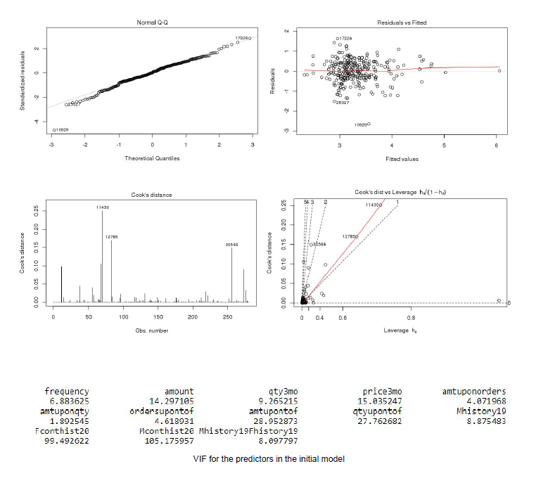
To evaluate the performance of our model, we ran the necessary checks for the main underlying assumptions of any good multiple regression model: normality, homoscedasticity, no outliers/influential observations, and no evidence of multicollinearity. The Q-Q plot of our model confirmed the assumption for normality, as the quantiles for the standardized residuals and theoretical quantiles largely followed a straight-line pattern. There were a few outliers observed in the Q-Q plot. The plot for residuals vs. fitted values confirmed the assumption for homoscedasticity, as no relationship was shown between the residuals and the fitted values. For outlier detection, the formula 4 / (n-(p+1)) yielded a threshold of 0.015. This threshold identified too many observations as outliers, so we decided on a threshold of 0.1 for Cook’s Distance, which removed 4 outliers, giving us a training sample of 276 observations. To check for evidence of multicollinearity among predictors, we looked at the Variance Inflation Factors for the variables in this model. The variables price3mo, amtupontof, and qtyupontof exceeded the VIF threshold of 15 as did the amount and frequency variables for Contemporary History.
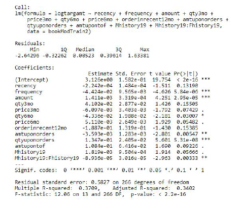
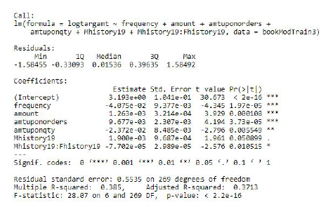
We re-ran the model for multiple regression after removing outliers and not including the variables with a VIF exceeding 15. The final multiple linear regression model found the following variables as statistically significant at the 5% level: frequency, amount, amtuponorders (amount divided by the total number of orders), amtuponqty (amount divided by total number of books ordered), the amount variable for the History category (p value = 0.05089), and the interaction between the amount and frequency variables for the History category.
This final model has an R-squared of 0.385, and an adjusted R-squared of 0.3713. The model details and diagnostics for the final model is illustrated in Figure 9.
One final check we performed to test our model involved exploring the spread of the test data. In order to optimize our model, we had previously removed outliers in the training set where amount upon order was larger than 1000, quantity upon order was larger than 40, and amount upon quantity was larger than 60. We observed similar outliers in the test set, with values well above these previously defined thresholds for the aforementioned predictors. Wishing to preserve the integrity of the test data set, we decided to keep these observations but to impute a predicted value for them. We made this decision through observation of the wildy large predicted values created when predicting the target amount for these customers using our multiple regression model (on the order of 10e40 or greater). Therefore, we chose as our imputed predicted value the maximum observed target amount for the training data. If we had left the massive predicted values in the model, our overall standard error would have been erroneously massive. Additionally, since we had removed the corresponding outliers in the training set, the model is unable to anticipate such extreme cases, so our imputation was absolutely necessary here, since we had endeavoured to include all observations in the test set. Furthermore, we justify our removal of the corresponding outliers in the training set by the increase in R2 of our model following their removal. In total, only 2 such observations (0.007873% of the testing data) were found with the aforementioned outlier characteristics. Although this imputation was relatively minor with relation to the size of the test data set, its effect was appropriately large due to the extremeness of the outliers.
MODEL VALIDATION
STATISTICAL SIGNIFICANCE
The predicted target amount for customers with previous order data (time on file > 0) in the test set was calculated directly from our predictive models: E(log target amount) = the product of the probability of logtargamt > 0 given by the logistic regression (after adjusting for oversampling) and the predicted logtargamt value given by the linear regression. For the customers in the test set with time on file = 0, we artificially created values that, to the best of our ability, mimic the predictions given by the logistic and linear models if previous order data had been logged. As stated in the previous section, the probability of logtargamt > 0 for these customers was imputed as 0.5287 (the overall response rate in the training set). Similarly, the predicted logtargamt value that should have been found in the linear regression was imputed as the mean value of logtaramt among new users from the training dataset. E(log target amount) was calculated for these new customers in the test set by multiplying these two values together to get an artificially predicted target amount. This product, the predicted log target amount, was then exponentiated and subtracted by 1 to obtain the predicted target amount. The RMSE of our final model is $10.57, suggesting satisfactory model performance.
FINANCIAL SIGNIFICANCE
Using our predictive model, we identified the customers with the top 500 predicted target amounts. The sum of these predicted purchases totals $2,261.83. Their total actual purchases totaled $6,449.529, which represents the payoff of our predictive model. After noting the accuracy of our prediction compared to the payoff (35.07% of the actual payoff), we focused on the true financial criterion - the payoff percentage. We pinpointed the 500 customers who actually had the highest purchased amount during the promotional period. Their purchases totaled $27,035.11. Therefore, our payoff percentage is 6449.529/27035.11 = 23.85%. This result indicates that even though our logistic and linear model both have high accuracy and R-square in predicting the response variable, there is still space for improvement in terms of actual performance.
The payoff percentage of 23.85% gives one measure of our model’s accuracy at predicting the purchase amount of the top 500 prospects; however, we decided to further optimize the financial success of our model by finding the number of prospects which maximizes the short term profit. With the assumption that the profit margin is 25% of the purchase amount, we maximized 0.25 * (sales revenue from the top x predicted prospects - 1 * x to yield 852 as the optimum number of top prospects to target, giving a short term profit of $1,319.74. A logical next step involves calculating the payoff percentage for the top 852 customers and compare it to the percentage for the top 500 customers. This percentage was slightly higher: 25.96% for the top 852 vs. 23.85% for the top 500. Since the difference is not much, we can say that per the results, majority of the maximum probable profit can be achieved by targeting the top 500 customers. Future exploration of financial accuracy could illuminate better ways to optimize fiscal payoff; however, this is not in the scope of our project.
CONCLUSION
In our final models, purchase frequency and the interaction of amount and frequency for the History category were significant in both classifying responders and predicting order amounts for responders. A multitude of predictors were significant in classifying responders or non-responders, including the original variables recency, frequency, and time on file, time-sensitive variables for purchase behavior over different time periods, and certain categorical variables, in addition to interactions among variables. For predicting order amounts for responders, a smaller subset of variables, including frequency, amount, amount per order, amount per book brought, and the History categorical variables proved significant. The root mean squared error of the predicted target amount was $10.57, indicating statistically strong final models. The total purchases of our top 500 predicted amounts fell a bit short of the total orders to the actual top 500 customers, at a 23.85% payoff percentage.
We felt that more information about this particular promotion could have helped our prediction accuracy. If we had known whether this promotion was general or specific to certain categories, our categorical variable analysis would have become more efficient. Also, promotion implementation was unclear: if the promotion was for a certain percent off one order, this would have incentivized different ordering behavior than a promotion that would apply to all orders. Additionally, information regarding promotional audience (e.g. whether it went out to all customers, a random sample of customers, or targeted groups of customers) would have also been beneficial. Another possible metric of success for a promotion could have been how many customers engaged with the promotion (e.g., clicked through an e-mail vs. deleted it), but didn’t ultimately purchase. Further potentially beneficial metrics, such as frequency and amount of time spent on the book store’s website, as well as what they typically do while browsing the website, could have also improved our model. Finally, customer service information may have also been beneficial. A customer who frequently engages customer service representatives could be more likely to purchase. However, negative recent experiences could decrease the probability of future purchases.
TEAM MEMBERS
LINKS
REFERENCES
- Tamhane, Ajit C. Predictive Analytics: Parametric Models for Regression and Classification Using R. (Wiley Series in Probability and Statistics)


Leave a comment