
Luxury European Hotels: Predicting Guest Review Scores Based on Hotel Reviews
The goal of this analysis was to predict the score, on a scale from 1 (lowest) to 10 (highest) that a reviewer will give after a stay at a luxury hotel in one of six European cities.

In order to generate our predictions, we examined a set of 515,738 reviews with data about the hotel, the reviewer and some elements of the review besides the score, which we augmented by parsing text tags, transforming features, and pulling in outside weather data. We fit the resulting data with several supervised learning models to generate a predicted score for each review. Gradient boosting trees provided the best fit for our data, accounting for 42.8% of the variance of reviews in our test set. We found that, unsurprisingly, the ratio of positive words to negative words in the review was the strongest predictor of the reviewer score. Other important predictors were the distance from the city center, the total length of the review and the high and low temperatures for the day of the hotel visit. Our primary conclusion was that factors available outside of the review provided limited predictive power as to how a reviewer would respond.
INTRODUCTION
As our world becomes increasingly digital, more and more consumers are relying on online reviews to help them decide what to buy, where to travel, and where to stay. Especially in the hotel review industry, these online customer reviews can make or break a business. According to surveys conducted by Trip Advisor and Trust You [4]:
- 88% of travellers filter out hotels with an average star rating below three [on a scale of one to five]
- 32% eliminated those with a rating below four
- 96% consider reviews important when researching a hotel
- 79% will read between six and 12 reviews before making a purchase decision
- Four out of five believe a hotel that responds to reviews cares more about its customers
- 85% agree that a thoughtful response to a review will improve their impression of the hotel
We have a dataset from Kaggle, originally scraped from Booking.com, with information on 515,738 reviews covering 1,493 unique luxury hotels in Europe. We will be predicting the rating that each user will give a particular hotel based on a stay. We will identify how different attributes of each hotel and each customer impact the review score, and identify whether a particular type of customer has a propensity to provide a positive or a negative review. Our analysis can help a hotel identify its loyal group of customers and the areas of service in which it excels. This can help drive future rebranding, marketing and customer service strategy and also help identify gaps where a hotel could potentially improve.
DATA CLEANING AND EXPLORATORY DATA ANALYSIS
DATA OVERVIEW
The original dataset included 17 different variables. Each reviewer leaves certain pros and cons for a particular hotel and a rating for the hotel from 1 (lowest) to 10 (highest). We also had additional information, which fell into three broad categories: hotel specific information, guest specific information and stay or review specific information. The variables are listed below:
Hotel Specific Information:
| Field | Description |
|---|---|
| Hotel_Name | Name of the hotel |
| Hotel_Address | Address of the hotel |
| lat | Latitude of the hotel location |
| lng | Longitude of the hotel location |
| Total_Number_of_Reviews | Total number of valid reviews that a hotel has been given on booking.com |
| Additional_Number_of_Scoring | There are also some guests who just made a scoring on the service rather than a review - This number indicates how many valid scores a hotel has without a review |
| Average_Score | Average score of the hotel, calculated based on the latest comment in the last year |
Reviewer Specific Information
| Field | Description |
|---|---|
| Reviewer_Nationality | Nationality of the reviewer |
| Total_Number_of_Reviews_Reviewer_Has_Given | Number of reviews the reviewer has given in the past on Booking.com |
Stay Specific Information
| Field | Description |
|---|---|
| Reviewer_Score | Score the reviewer has given to the hotel, based on his/her experience (this is the response variable in our models) |
| Negative_Review | What the reviewer wrote in the “negative” or “cons” section of the review |
| Review_Total_Negative_Word_Counts | Total number of words in the negative review section |
| Positive_Review | What the reviewer wrote in the “positive” or “pros” section of the review |
| Review_Total_Positive_Word_Counts | Total number of words in the positive review section |
| Tags | Tags reviewer gave the hotel |
| Review_Date | Date when reviewer posted the corresponding review |
| days_since_review | Duration between the review date and scrape date |
EXPLORATORY DATA ANALYSIS AND FEATURE ENGINEERING
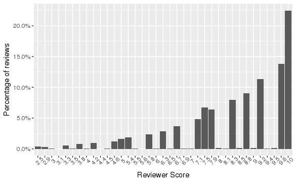
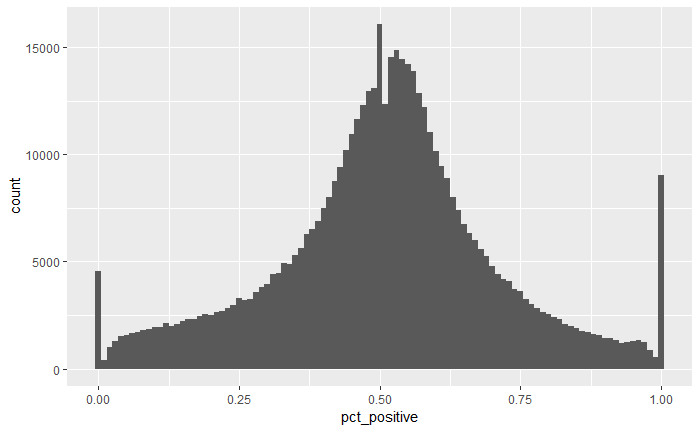
As shown in Figure 1 below, our response variable was fairly well distributed and covered a wide range of the rating scale, with a minimum score of 2.5 and a maximum of 10.
Based on the variables available to us, we focused on 4 distinct feature groups:
- features of the guest
- distinct perks of each hotel
- outside factors that could affect the customer’s stay
- features of the review text itself
To determine a hotel’s “usual” guest, we used the customer tags related to each stay. The tags included information such as whether the trip was for leisure or business, whether the guest was traveling with a family, the length of stay, and the type of room. We started by aggregating these at a hotel level to assign tags to the hotels. We only aggregated the tags from highly rated reviews so the tags would be indicative of that hotel’s particular expertise. We then used TF-IDF (Term Frequency - Inverse Document Frequency) to determine the importance of each tag, by using each tag as a term and the hotel’s aggregated tags as the document. We ended up with 7 broad categories: trip type, room type, luxury room type, view type, access type, time of stay, and whether the guest was provided free services. For each of these categories, every hotel was assigned its top tag, i.e. tags for which it received great reviews. Once we had the hotel tags, we created a compatibility score variable that captured hotel and customer compatibility. We assigned the customer tags to each of the 7 broad categories. We then compared the customer tags to the hotel tags for each of the categories, adding one to the compatibility score for each tag that matched.
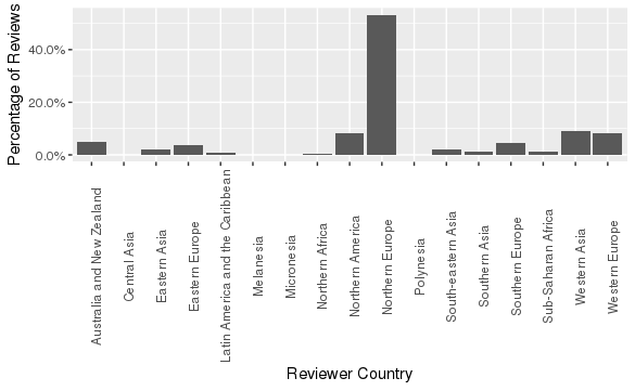
Another feature we created about each guest was whether a customer was a tourist. We defined “tourist” as a customer who was not from the same country as the hotel. If the hotel’s address matched the customer’s nationality, the customer was not marked as a tourist. We also analyzed the home country of each guest. As we had 227 unique countries, we decided to aggregate these into 18 sub-regions. Figure 2 shows the percentage of guests from each sub-region.
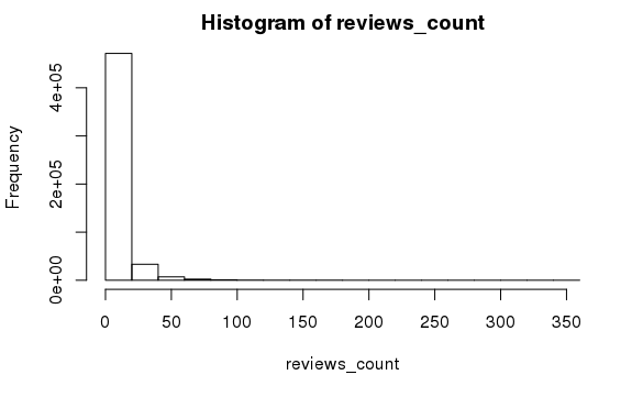
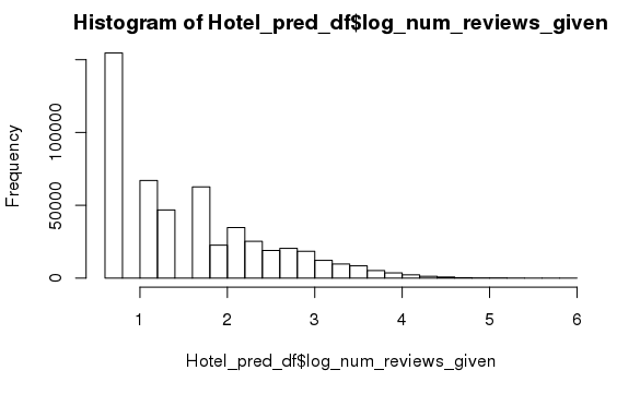
Finally, we used the number of reviews given by a reviewer as a feature as well. We log transformed this variable as this was heavily right skewed, as you can see from the histogram below.
Secondly, we analyzed the perks of each hotel. The first variable we created was the hotel city, which we extracted from the address. The hotel reviews take place in the following six cities:
| Vienna, Austria | Paris, France | Milan, Italy | Amsterdam, Netherlands | Barcelona, Spain | London, United Kingdom |
|---|---|---|---|---|---|
| 38,939 | 59,928 | 37,207 | 57,214 | 60,149 | 262,301 |
| 8% | 12% | 7% | 11% | 12% | 51% |
We also thought it would be interesting to have a feature which notes the distance from the city centre. A consistent characteristic of European cities is a central city centre that is also a public transportation hub. We hypothesize that hotels closer to the city centre would receive a higher rating as this would improve the guest’s overall experience due to accessibility and proximity to tourist destinations.
Additionally, we focused on external factors affecting the quality of a stay. We hypothesized that the weather could affect whether a stay was pleasant. To create these features, we pulled historical weather data for each review using the Dark Sky API (darksky.net/dev), based on the hotel city and the review date (as a proxy for the stay date). We created features from the high and low temperature. We also used the summary to find the most common types of weather, and created a weather summary feature with 7 factors: breezy, clear, cloudy, foggy, humid, rain, and snow.
Finally, we focused on features of the review itself. Our original data included the text and word count of the user review split out into positive and negative sections. We calculated a sum of the word counts from these positive and negative review sections then log-transformed that aggregate count, to correct for the heavily right-skewed distribution. In order to summarize the ratio of positive to negative words in the review, we generated the pct_positive variable, which is the percent of total review words in the positive section. We weighted this towards the middle for reviews with fewer than 50 words, under the assumption that people who wrote fewer words potentially felt less strongly than those who wrote more words. We weighted percent positive using the following formula:
pct_positive = (positive word count ÷50) - (total word count ÷100) + 0.5
To summarize, the final features we used to fit our models are listed below:
Customer Features
| Feature | Description |
|---|---|
| tourists | A person is a tourist if his home country does not match his country of stay |
| Reviewer_sub_region | Home region of the reviewer, aggregated into sub-regions |
| log_num_reviews_given | Log of number of reviews given by the particular reviewer |
| access_type_cust | Access type provided to the customer, eg. pool access, spa access |
| accessibility_cust | Accessibility of the room |
| free_cust | Any free services provided to the customer |
| other_cust | Miscellaneous room/hotel features |
| other_room_types_cust | Luxury room or not |
| room_type_cust | Non-luxury room type that the customer stayed in |
| time_of_stay_cust | Length of stay |
| trip_type_cust | Type of trip that the customer was on, e.g. business or leisure |
| view_type_cust | Whether or not the guest’s room had a view |
| CommonScore | Compatibility score for customer and hotel |
Hotel Features
| Feature | Description |
|---|---|
| access_type | Most favoured access type |
| accessibility | Whether accessibility rooms are available |
| free | Top free service provided by the hotel |
| other_room_types | Luxury room available or not |
| room_type | Top standard room available in the hotel |
| time_of_stay | Favoured length of stay (short or long) |
| trip_type | Top trip type for the hotel |
| view_type | Whether rooms with views are available |
| City | The city in which the hotel is located |
| distance | The distance of the hotel from the respective city’s city centre |
External Features
| Feature | Description |
|---|---|
| TempHigh | The high temperature on the date the review is submitted |
| TempLow | The low temperature on the date the review is submitted |
| weather_summary | Categorical variable describing the weather on the date of review |
Review Features
| Feature | Description |
|---|---|
| pct_postive | The percent of total review words in the positive section of the review, weighted toward 0.5 for reviews with low total number of words |
| log_review_word_count | Combined positive and negative word counts, under a log transformation |
MODEL FITTING AND VALIDATION
TRAIN AND TEST SETS
Since our dataset had over 500,000 observations, performing cross validation on such a large dataset would be very computationally expensive. We therefore split our dataset into a train and test set using random sampling. Our data set was also large enough that we expected we would not overfit on the training data. The train set contained 75% of our dataset, and the remaining 25% was included in the test set.
BASE COMPARISON
As a pure base comparison, we used the average score for each individual hotel in our dataset as the prediction for the Reviewer Score. Using our entire dataset, this gave an R-squared of 13.74%.
LINEAR REGRESSION MODEL
We then started out by fitting a linear regression model. We had several categorical variables, but we decided to use this model as a base to compare to our other models. Our first step was to fit the full model, which yielded a training R-squared of ~33%. We checked the residual plots for the full model linear regression and noticed that the residuals were neither very normally distributed and nor were they random. We then ran a stepwise regression to see if a smaller model would be a better fit. This step dropped 4 variables, keeping the R-squared at ~33%. The most significant predictors were hotel location, number of reviews given, temperature, a couple of hotel related tags and customer tags. Our final linear regression model had 24 predictor variables, a training R-squared of 33.14% and a test R-squared of 32.57%.
SIMPLE REGRESSION TREE
Next we fit our data using a simple regression tree. We used this model as our data has numerous categorical variables, and trees are one of the best ways to handle categorical predictors. The simple tree output is shown below. (Note that some of the variable names have been shortened to fit on the plot).
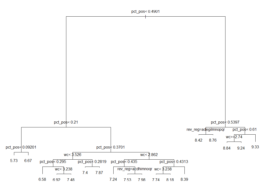
As you can see from the plot above, there are three predictors this tree kept: pct_positive, log_review_word_count, and Reviewer_sub_region. As expected, the percent of the words in the review that were positive had the largest effect on the response, and the less positive the review was, the lower the score. Percent positive was 21 times more important than the next variable. Word count was next most important, and then finally the home country of the reviewer. In the first split on Reviewer_sub_region, the tree indicated that guests from the following countries give slightly lower reviews: NA, Eastern Asia, Eastern Europe, Melanesia, Northern Africa, Polynesia, South-eastern Asia, Southern Asia, Southern Europe, Sub-Saharan Africa, Western Asia, and Western Europe. Guests from the following sub regions thus give slightly higher reviews: Australia and New Zealand, Central Asia, Latin America and the Caribbean, Micronesia, Northern America, and Northern Europe. The other split on Reviewer_sub_region gave a similar split, however Central Asia and Micronesia give lower reviews in this split and Eastern Europe, Melanesia, and Sub-Saharan Africa give higher reviews.
The model had a training R-squared of 35.48% and a cross validated R-squared of 35.37%. Running multiple replicates of cross validation, the model had an R-squared of 35.35%. Finally, using the model to predict for the test set resulted in an R-squared of 34.75%. This was very close to the training R-squared, indicating that our model is not overfitting on the training data. If we used a slightly lower initial complexity parameter (.0001 instead of .001), the R-squared was slightly higher at about 37%. However, the tree was then very large (even with pruning back to a complexity parameter within one standard error) and lost all interpretability. We therefore used the more interpretable model with the slightly lower test R-squared of 34.75%. This R-squared is slightly higher than the test R-squared of the linear model, which is 32.57%.
GRADIENT BOOSTED REGRESSION TREE
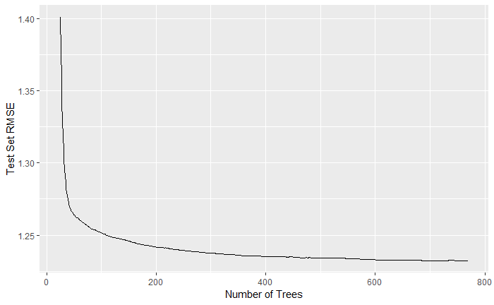
We then fit a boosted tree model using the XGBoost package in R. We chose this package as opposed to the gbm package from class due to the significant increase in speed and inline use of parallel processing, allowing for significantly faster fitting of our models. While fitting the model we chose the appropriate number of trees to grow and how large of trees to grow by assessing the prediction R-squared.
The model-fitting process involved building different models using our training data with different values for various parameters and tracking the performance of each model against the test data. The primary tuning parameters we worked with were the shrinkage parameter (eta in the XGBoost package) and how large to build the individual trees (controlled by the max_depth parameter). We were able to assign a large max number of trees (typically 5000) and the xgb.train function would identify the tree with the lowest RMSE over the test set. After tuning these parameters, using the cross section of shrinkage parameters between 0.01 and 1 and tree depth from 2 to 7, we found the best model used a shrinkage parameter of 0.1 and a tree depth of 6, fitting over 720 trees for a maximum test R-squared of 42.8%.
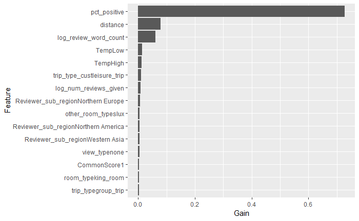
We used the xgboostExplainer package to delve into the specific effects of our most important variables on our boosted tree model. We first used the importance calculation within the xgb.train package to identify those variables that contributed the most predictive power. From the graph below, we can see that pct_positive was by far the most predictive feature, followed by distance and temperature during visit.
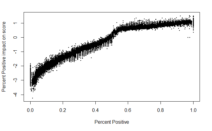
The xgboostExplainer then compiled the overall effect each feature had on each observation in the test data. Unsurprisingly, more positive reviews caused the model to predict higher scores, though the model was not quite linear, flattening out at the high end of the scale.
None of the other variables had nearly as well defined of a relationship with scores, though they can provide some insight as to the underlying relationships. The model appeared to predict higher scores for hotels closer to their respective city center, but it also appeared that this feature was isolating individual hotels, so we were probably accounting for some information outside of just distance in these effects.
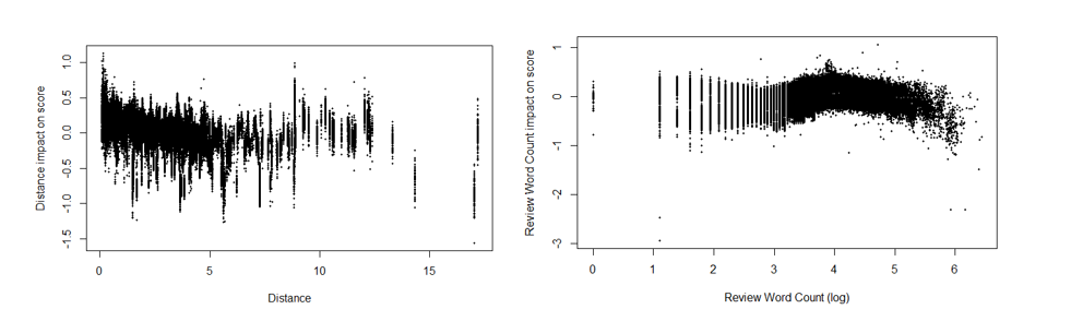
The total word count in a review stayed largely flat until a certain point then fell off somewhat with some significant negative effects in the high values.
RANDOM FOREST
We fit a Random Forest model on the training data to predict the Reviewer score. Since our dataset was very large, we decided to sample down our dataset to only using 10% of observations (38,661 observations) for hyperparameter optimization and model fitting. To tune the parameters, we used mtry(Number of variables randomly sampled as candidates at each split) as 5 and 10, and nodesize(Minimum size of terminal nodes) as 10 and 20. The optimum parameters were mtry = 5 and nodesize = 20 which provided the best OOB (Out of bag) R-squared of 37.82%. The ntree(Number of trees to grow) parameter was fixed at 100.
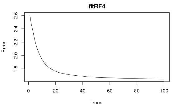
We used the above tuned parameters to fit our model. Since we used a 10% sample of our data, we decided to fit the model with the optimized parameters on 4 different samples to eliminate any random sampling bias. The out of bag R-squared results were 37.87%, 38.03%, 37.77% and 37.92%. We used each of these four models to predict the scores in our test set. Taking an average of those errors, we got a test R-squared of 38.60%.
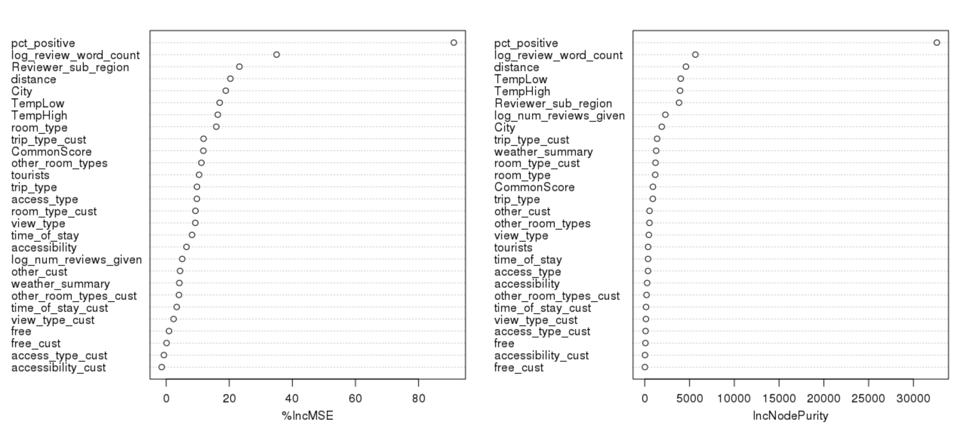
As we can see from the variable importance plot above, the most variable which explained the most variance was the percent of positive words in the review given. The length of review word count and the reviewer sub-region also impacted the review score by a significant amount. These three variables were the same ones that the simple tree model found to be important. The other important important variables are hotel city, distance from city center, and temperature. Below are the main effects plots for some of the most important variables:
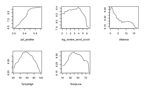
- Pct_positive: As expected, the higher the percentage of positive words in the review, the higher the review score
- Log_review_word_count: The longer the review is, the more likely it is that the reviewer score will be low. We can conclude that negative reviews are generally longer than positive reviews.
- Distance: As the distance of the hotel from the city center increases, the Reviewer score decreases. This shows that the location and surroundings of the hotel also matters to customers
- TempHigh and TempLow: Both the TempHigh and TempLow chart show the same story. As the temperature becomes colder or hotter, the probability of a positive review reduces.
MULTIVARIATE ADAPTIVE REGRESSION (MARS)
MARS is an alternate approach to capture non-linearity of a model by assessing cutpoints (knots) similar to step functions. The procedure fits multiple linear models to each dataset, one line for each knot. The following example from UC Business Analytics shows graphs for one knots and two knots:
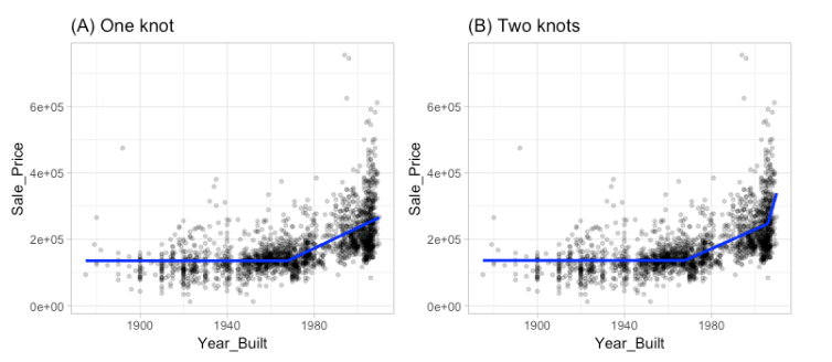
The procedure can be fit until many knots are found. However, choosing the number of knots again comes down to the bias-variance trade-off present in the rest of our models. If we fit a higher number of knots, the variance will be high and the bias will be low (and will also lead to overfitting).
We fit a MARS model on the training data using the earth package. By default, the function will prune to the optimal number of knots based on an expected change in the R-squared of the training data. This calculation is performed by the Generalised cross-validation procedure (GCV statistic). For our data, we started by fitting a simple model with no interactions and we had a train R-squared of 36.04% and a test R-squared of 35.48%.
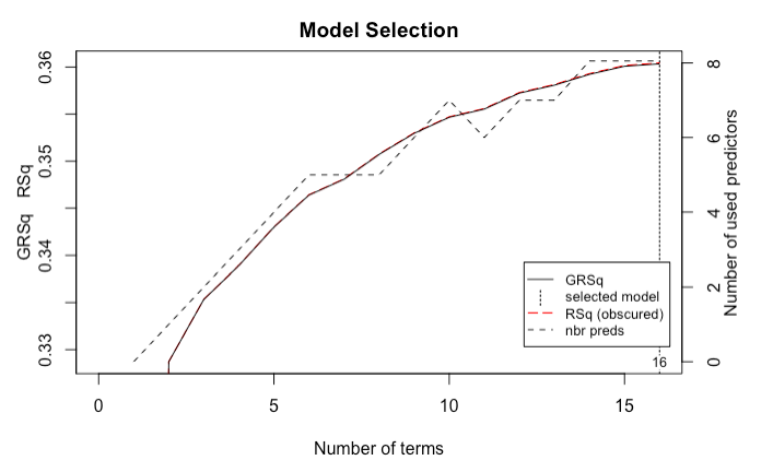
We also tried to include higher degree = 2,3,4 (interactions) in our model but it did not improve the model significantly and was computationally more expensive.
The earth package also includes a backward elimination feature selection routine that looks at reduction in the GCV estimate of error as each predictor is added to the model. This total reduction is used as the variable importance measure. The variable importance chart is below:
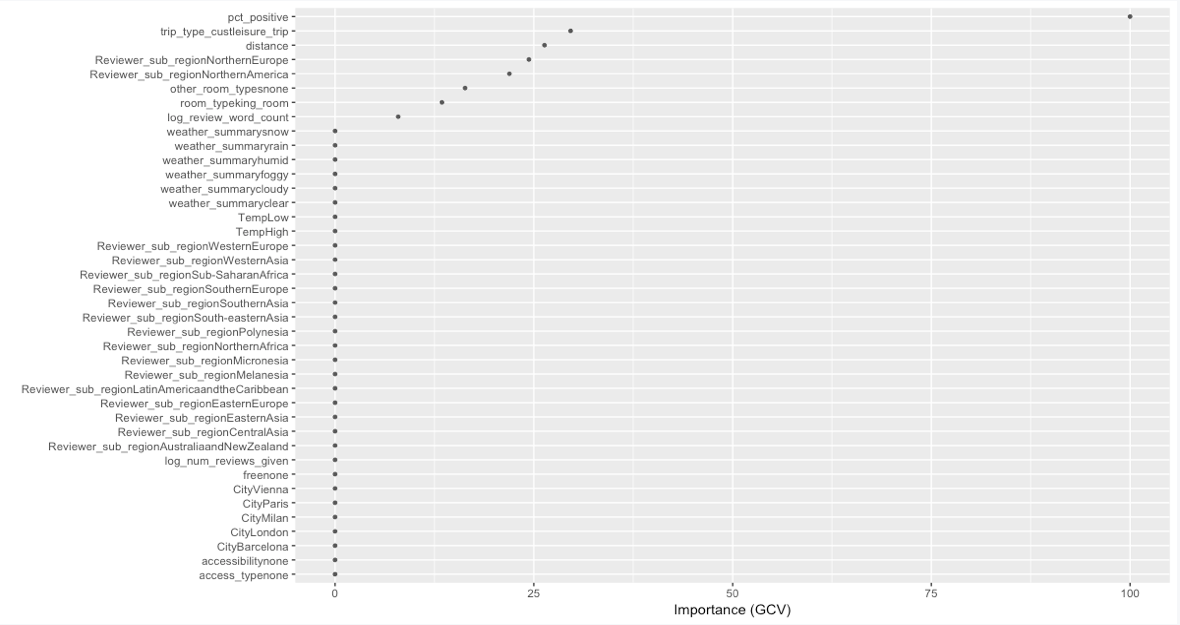
The result was very similar to our previous models with pct_positve as the most important predictor. The other important variables are: trip_type, distance, reviwer_sub_region, room_type, and word_count in a decreasing order.
OTHER CONSIDERATIONS
We also considered a slightly different analysis. We were interested in predicting the review score without using any of the variables about the actual review, i.e. removing log_review_word_count, percent_positive, and log_number_reviews_given from our predictor set. This will give a prediction based on only the things the hotel will know about a guest the moment they walk through the door, such as nationality of reviewer, the weather, and whether the customer is on a business trip. This would help a hotel consider how to treat each individual guest, perhaps by recommending different amenities, or providing additional services to guests traveling with young families. However, these models did not perform very well. We ran a simple tree model, and using a very low initial complexity parameter, our test R-squared was 9.5%. This is worse than even the base model R-squared of 13%, which just used each hotel’s average score as a prediction for Reviewer_Score. We therefore focused on the original analysis which includes the review variables.
CONCLUSION
In conclusion, gradient boosted tree model was the best at predicting the Reviewer Score. This model had the highest test R-squared of 42.8%, compared to Random Forest (38.60%), MARS (35.48%), Simple Tree Regression (34.75%), and the Linear Regression (32.57%). Unsurprisingly, in all of the models, pct_positive was consistently the most important predictor. The Boosted Tree model also found that the total word count in a review had significant negative effects on the review score at very large word counts. The distance from the city centre was also an important variable, however, we believe this may have been a proxy for the individual hotel, and capturing other effects rather than just distance. Finally, both the Boosted Tree and the Random Forest models found that guests did not like extremely hot or cold temperatures.
We would have liked to have had a more powerful predictive model when using only the guest and hotel features, and none of the review information. It would also have been interesting to have had a Reviewer ID variable, so we would have been able to ipsatize the ratings, to account for users who rate everything very high, or rate everything very low. Additionally, some more demographic information about the reviewers could have helped to improve the predictions.
TEAM MEMBERS
LINKS:
REFERENCES
- Dark Sky, darksky.net/dev
- Liu, Jason. “515K Hotel Reviews Data in Europe.” Kaggle, 21 Aug. 2017, www.kaggle.com/jiashenliu 515k-hotel-reviews-data-in-europe
- “Multivariate Adaptive Regression Splines.” Multivariate Adaptive Regression Splines · UC Business Analytics R Programming Guide, uc-r.github.io/mars
- “What Impact Do Guest Reviews Have on Hotel Bookings?” SiteMinder, 21 June 2017, www.siteminder.com/r marketing/hotel-online-reviews/influence-travellers-reviews-hotel/


Leave a comment